Solving for sensor orientations and cable delays in DIMENSION4
The solver tab
The solver is available in LSC on the Solve sensor parameters tab. The solver manages the process of setting up correct sensor orientation and cable delay timing values. The panel at the top of the solver tab gives an overview of sensors' solver status, and you should aim for all sensors to have 'OK' results for orientation and cable delay timing.
Sensors are collected together by group. Group summaries show the worst case results for sensors in the group. For example, if any sensor does not have a result, the group summary is “Incomplete”.
If all sensors have results but one is “Poor”, the group summary will be “Poor” as well.
Prerequisites for using the solver
The solver requires some configuration steps to be completed in order for it to work:
- Configure logging – set up the logging server that gathers and distributes data from the sensors. If this step is not done then the solver will not receive any data from sensors. See Configuring Logging.
- Place sensors – add sensors with the correct positions, optionally adding estimated orientations (the estimated orientations can also be used instead of solver results if you decide that hand-measured orientations will be better for a particular sensor). If this step is not done then the solver will be unable to calculate orientations or cable delays. See Adding and Placing Devices.
- Configure timing – set the timing source flag for the timing source sensors. If this step is not done then the sensor network will not generate any data. See Configuring Timing.
How to use the solver to calculate orientations and cable delays
To calculate a new set of results, place a tag in a suitable position, and do this sequence of steps:
- Click 'Solve', enter the tag id and location, and wait for sensors to appear in the list.
- Tick sensors if and only if you know they have a direct line of sight to the tag.
- Wait for the timing results to include all the pairs of sensors that you expect.
- Reject individual results for yaw, pitch or cable delay if you don't want them to be considered by the solver (for example, if pitch values look wrong due to multipath effects). The system will use the best accepted results to set orientation and cable delay values.
- Click 'Save' to store results. Clicking 'Save' again overwrites previous results for a solver run.
- Click 'Close' to end the solver run. If you clicked ‘Save’, it will appear in the list.
- Inspect old solver runs (and change accept/reject decisions) by double-clicking on them.
How to assert that infrastructure has changed
The solver keeps track of all the solver runs done, and how they were used to calculate sensor properties, so it must be told about any changes in infrastructure that may affect the calculations.
Use the Replace infrastructure tab to tell the system about sensor swaps, sensor position changes and cable swaps done after any solver runs have been saved.
- Sensor swaps do not invalidate any results. The label in the UI will show both MACs if and only if the sensor doesn’t have a name. Results will automatically apply to the new sensor.
- Sensor moves invalidate all orientation results for the sensor.
- Cable swaps invalidate all timing results for sensors with the cable in the timing route.
It is possible to retract any of the assertions above, in which case previously invalid solver run results may become valid again.
Background information for advanced users
How the solver works
The solver takes some preconditions, and some measurements, and uses these values to calculate possible values for sensor yaw angles, pitch angles, and cable delays. So each solver run represents a function that transforms preconditions and measurements into calculated sensor properties, as shown below:
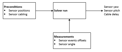
By storing the solver runs and combining their results together, the solver is able to work out the optimum values for the pitch, yaw and cable delay of each sensor and to keep track of the sensors that have been solved and the calculation steps used in the process.
Sometimes the preconditions to a solver run can change. When a sensor is moved, a timing cable is replaced or the timing tree is reconfigured, some of the results of some solver runs are no longer valid. The system will mark these values as Invalid.
Sometimes a solver run might not give good answers for all its results, so the user is able to reject them via the user interface (see steps 4 and 7 above). The system will mark these values as Rejected.
A result that is Invalid or Rejected is called an unused result. A result that is neither Invalid or Rejected is called a candidate result. The solver will consider all candidate results and typically use the result with the lowest variance.
Detailed operation of sensor orientation setting using the solver
How orientations are stored
The Sensor placement component sets the value of 'Sensor/Physical/Estimated Position', which has translation and orientation components.
The configuration server sets ‘Sensor/Physical/Position’. The translation component is taken straight from the estimated position, because this should have been surveyed and is assumed to be correct. The orientation component is taken from solver results for orientation or from the estimated orientation if there are no candidate results.
Calculating the final orientation result
Unused orientation results are stored persistently (they might become candidate results later). While unused, they do not affect ‘Sensor/Physical/Position’ and are labelled with “Invalid” and/or “Rejected” in Solve sensor parameters.
Orientation results are not used in the following cases:
- The sensor has been deleted.
- The result is Rejected, because the ‘Accept?’ checkbox is un-ticked in Solve sensor parameters, either when saving for the first time or retrospectively.
- The result is Invalid, because there is an assertion in Replace infrastructure that the sensor has moved after the solver run.
Of the candidate results, the result with the lowest variance is used.
To get an orientation result with summary “OK”, there must be candidate results with the following:
- Yaw std dev < 2° from 100 or more measurements
- Pitch std dev < 4° from 100 or more measurements
Otherwise, the orientation summary for the sensor will be “Poor”.
How to set an orientation manually
If there are any candidate results for a sensor pitch or yaw then one of them will be used as the actual pitch or yaw of the sensor. Therefore, to set a sensor orientation manually, use Place devices to estimate the orientation and do not accept any orientation results for that sensor. This will give a sensor summary of “Not done” and a group summary of “Incomplete”.
Detailed operation of sensor cable delay setting using the solver
How cable delay results are stored
Configure timing sets ‘Sensor/Physical/Timing/Source’, which is true or false.
The configuration server sets ‘Sensor/Physical/Timing/Acting Source’. The value is taken straight from the user-assigned flag.
Once the sensors have been cabled together and have booted, after a few seconds a sensor reports its timing upstream sensor and the output port from which it receives the timing signal. This is stored in 'Sensor/Physical/Timing/Upstream Sensor' and 'Sensor/Physical/Timing/Upstream Port'.
The system will automatically determine every sensor's current timing tree root, based on the timing topology information (upstream sensors) and the acting timing source information. The timing tree root is stored in 'Sensor/Physical/Timing/Current Root'. When performing TDOA calculations, everything is dealt with in terms of the sensor's timing tree root.
Timing results from solver runs are stored in pairs of sensors. Results include the delay and variance. A graph of delay/variance values is computed for all sensors that have timing results. The configuration server sets ‘Sensor/Physical/Timing/Root Cable Delay’ to equal the sum of delay values along the path from its current root that has the lowest total variance.
Calculating the final cable delay result
Unused timing results are stored persistently (they might become candidate results later). While unused, they do not affect ‘Sensor/Physical/Timing/Root Cable Delay and are labeled with “Invalid” and/or “Rejected” in Solve sensor parameters.
Timing results are not used in the following cases:
- The sensor has been deleted.
- The result is Rejected, because the ‘Accept?’ box box is not checked in Solve sensor parameters, either when saving for the first time or retrospectively.
- The result is Invalid, because there is an assertion in Replace infrastructure that a cable within the route to the timing source has been changed after the solver run.
- The physical timing route has changed.
The remaining results are candidate results. The candidate timing results with the lowest variance are used.
To get a timing result with summary “OK”, there must be candidate results for pairs of sensors that form a route from a timing root to the sensor with the following:
- Total variance < 1
To get the group summary “OK”, all the sensors in the group that have the same physical timing root must have timing results connecting them. When this is not the case, the timing result is appended with the “partition” number and the summary is “Incomplete”. To fix this, accept timing results between sensors from each partition.
How to set a cable delay manually
You can set the 'Root Cable Delay Override' value to manually set the Root Cable Delay, in which case the sensor summary will say “Overridden”. In this case, the group summary can still be “OK” because it is assumed the user is a developer doing testing—there is no way for users to estimate cable delays.
Cable delay result worked example
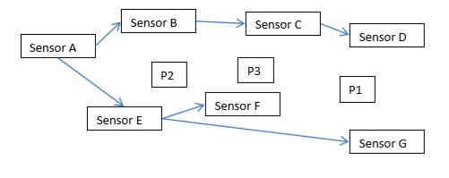
- Sensor A is the Timing Source, and after upstream sensor information has been reported it will be automatically set as the 'Current Root' for all the other sensors. The Root Cable Delay for Sensor A will be set to 0.
- The cable delays are solved with the tag at P1 first (note there is no need to necessarily start near the timing source). We get results from sensors C, D, and G. This means that we get the following results:
- C-D delay
- D-G delay
- C-G delay
- The system cannot calculate any cable delays from the Current Root sensor to any other sensor yet.
- We then solve with the tag at P2, getting results from A, B, E and F:
- A-B delay
- A-E delay
- A-F delay
- B-E delay
- B-F delay
- E-F delay
- The system can calculate the cable delay from the Current Root (sensor A) to sensors B, E and F:
- Root Cable Delay for B = delay A-B
- Root Cable Delay for E = delay A-E
- Root Cable Delay for F = delay A-E + delay E-F
- We then solve with the tag at P3, getting results from B, C, and F.
- The system can calculate the remaining cable delays:
- Root Cable Delay for C = delay A-B + delay B-C
- Root Cable Delay for D = delay A-B + delay B-C + delay C-D
- Root Cable Delay for G = delay A-B + delay B-C + delay C-G
- The Root Cable Delay for G calculation does not use information that mimics the actual timing cable topology. The algorithm ignores the topology in favor of minimizing the 'cost' of the path, where 'cost' is the variance of the candidate measurements.
- The delays are presented as sensor pairs with the delay and standard deviation. The sensors are ordered by MAC address. So if sensor B had a MAC of 00:11:CE:FF:00:01 and A was 00:11:CE:FF:00:02, then the delay would be B-A (and the value would be negative).